Reinforcement learning (RL) is a subset of machine learning that deals with sequential decision-making. The key difference from supervised learning lies in the data assumptions: supervised learning assumes data is i.i.d. (independent and identically distributed), meaning samples are independent of one another. In sequential decision-making, however, each action influences subsequent samples—creating temporal dependencies and non-stationary data distributions that require fundamentally different algorithmic approaches.

The RL framework formalizes this as an agent interacting with an environment, receiving observations and rewards, and learning a policy that maximizes cumulative reward over time. This formulation naturally captures problems where actions have long-term consequences: robotics control, game playing, resource allocation, and recommendation systems.

The RL landscape encompasses numerous paradigms, categories, and algorithms, shaped by factors like data availability, simulation cost, and whether a dynamics model or reward signal is accessible. While most RL successes to date have been online and on-policy (more on that in part 2), this blog series focuses on offline RL—an interesting paradigm when real-world interaction is expensive, dangerous, or unavailable (e.g. autonomous vehicles).

What is Offline RL?

In standard (online) RL, an agent learns by interacting with an environment: it takes actions, observes rewards, and updates its policy through this feedback loop. Formally, at each timestep the agent is in state \(s_t\), takes action \(a_t\), receives reward \(r_t\), and transitions to state \(s_{t+1}\). The objective is to maximize expected discounted return:

$$J(\pi)=\mathbb{E}_{\tau\sim \pi}\left[\sum_{t=0}^{\infty}\gamma^t r_t\right]$$

This work well, but in real-world applications we often can't afford the luxury of extensive exploration. You can't let a robot randomly experiment with surgical procedures, or allow a self-driving car to learn collision avoidance through actual collisions.

The natural alternative is simulation—but simulation has its own drawbacks: it can be computationally expensive, struggles to capture complex real-world dynamics, and still leaves sim-to-real domain adaptation as an open problem.

So practitioners often turn to behavior cloning (BC), treating the decision-making problem as supervised learning: given state \(s\), predict the action \(a\) that an expert would take. This is simple and scales well—which is why most robotics and autonomous driving companies relied on it for years. But BC ignores the sequential nature of the problem: errors compound over time as the agent drifts into states the expert never visited, a phenomenon known as distribution shift or covariate shift.

Offline RL offers a middle ground. Like BC, it learns entirely from a fixed dataset of previously collected experience—no environment interaction required. But unlike BC, it retains the RL objective: maximize cumulative reward rather than simply mimicking demonstrations. This allows offline RL to potentially improve upon the behavior policy that generated the data, rather than just imitating it.

Note: the behavior policy \(\pi_\beta\) is whatever policy (or mix of policies) generated the dataset. It could be a human expert, a scripted controller, an earlier learned policy, or a combination of all three.

Why Offline RL and why not BC

Behavior cloning is simple and often effective when data is high-quality and near-expert. But real-world data is rarely so clean. Offline RL offers two main advantages:

• The ability to learn from suboptimal data.
• Stronger generalization through compositional and corrective reasoning.

Learning from Suboptimal Data

Real-world datasets are messy, they contain mistakes, failures, and suboptimal decisions. Behavioral cloning treats all data equally—if you clone noisy behavior, you get a noisy policy. Offline RL algorithms, by contrast, can extract optimal behavior by:

• Weighting actions by their learned advantages
• Propagating value information to identify which parts of trajectories are worth replicating
• Learning not just "what to do" but "what NOT to do" from failed attempts

Generalization

Generalization in offline RL is often discussed under the umbrella of "trajectory stitching," but this conflates several distinct phenomena. Let's be precise about what BC can and cannot do.

Type 1: State Generalization (Similar Unseen States) = Equal

The ability to handle an unseen state \(s^′\) that is similar to a training state \(s\). This type of generalization is largely a function of model architecture and optimization, and not BC vs Offline RL distinction. However untuned offline RL could be worse because the Q-functions (Bellman errors) is sharper and more unstable than simple Maximum Likelihood Estimation (MLE) used in BC.

Type 2: Action Generalization = Equal

The ability to output an unseen action \(a′\) that is similar to training actions when appropriate. Like state generalization, this depends primarily on the policy's function approximator rather than the learning paradigm.

Type 3: Compositional Generalization (Stitching) = Offline RL is better

The ability to compose fragments of suboptimal trajectories into a new, successful trajectory—combining parts of Trajectory A and Trajectory B to create Trajectory C, which was never observed in the dataset.

BC is trajectory blind. If it sees a suboptimal path \(A \to B \to \text{Fail}\) and another path \(B \to C \to \text{Goal}\), BC will likely learn the average action at \(B\). It does not know that the transition \(B \to C\) is "better" than \(B \to \text{Fail}\) unless you filter the data beforehand.

Offline RL excel at this. Through the Bellman equation, the high value of reaching "Goal" backpropagates to state \(B\). When the agent arrives at \(A\), the Q-function tells it to take the action leading to \(B\) specifically because \(B\) connects to the high-value path, effectively stitching \(A \to B\) (from trajectory 1) and \(B \to C\) (from trajectory 2).

Type 4: Corrective Generalization = Offline RL is better

The ability to recover if the agent drifts off the ideal trajectory.

BC suffers from Covariate Shift. If the agent drifts to a state not in the expert data, BC has undefined behavior, often leading to compounding errors.

Offline RL can handle this if the dataset contains suboptimal/recovery data. Offline RL can learn "this state is bad, do X to get back to high value regions," whereas BC might confusingly try to clone the "bad" behavior if it's present in the dataset.

How does Offline RL work

To really understand offline RL, let's reinvent it naïvely, discover the problems, and see how they motivate the three main algorithmic approaches.

A Naïve Approach:

Given a dataset \(\mathcal{D}=\{(s_t,a_t,r_t,s_{t+1})\}\) collected by some behavior policy \(\pi_\beta\), a natural idea is:

1. Train a Q-function on the dataset.
2. Use this Q-function to improve our policy (e.g., via DDPG or SAC).

Why not value function like in AC and PPO? Because value functions only tells us how good a state is, it doesn’t tell us which action to take without on-policy rollout. Q-functions allow us to evaluate and compare arbitrary actions directly from offline data, which what we need to improve the policy.

What Will Go Wrong:

The Q-function learns to estimate action values for the states and actions in the dataset. But the dataset doesn't cover all actions in all states. For state-action pairs outside the data distribution, our Q-estimates are unreliable—essentially hallucinated.

This wouldn't be catastrophic if the errors were random. But Q-learning uses a max operator:

$$Q(s_t, a_t) \leftarrow r_t + \gamma \max_{a'} Q(s_{t+1}, a')$$

The max preferentially selects overestimated actions. These overestimates then bootstrap into subsequent Q-updates, creating a positive feedback loop. Estimation errors don't just persist—they compound and explode.

The policy, trained to maximize Q-values, happily exploits these inaccuracies. It learns to select out-of-distribution (OOD) actions precisely because their Q-values are erroneously high. The result: a policy that looks excellent according to our Q-function but performs terribly in the real environment.

This is the core challenge of offline RL: distribution shift between the learned policy and the data-collection policy, compounded by bootstrapping.

Three main Approaches to Offline RL:

The field has converged on three main strategies to address this:

1. Value Pessimism: Penalize Q-values for OOD actions.
2. Policy Constraint: Keep the learned policy close to the behavior policy.
3. Avoiding OOD Actions: Avoid querying Q-values for OOD actions entirely.

Value Pessimism (e.g., CQL)

Conservative Q-Learning (CQL) tackles distribution shift by explicitly penalizing the Q-values of actions outside the dataset distribution.

The key idea: push down Q-values across all actions while pushing up Q-values for actions actually in the dataset.

$$\mathcal{L}_{\text{CQL}} = \alpha \left( \mathbb{E}_{s \sim \mathcal{D}} \left[ \log \sum_{a} \exp(Q(s, a)) \right] - \mathbb{E}_{(s, a) \sim \mathcal{D}} \left[ Q(s, a) \right] \right) + \mathcal{L}_{\text{TD}}$$

The net effect is that Q-values for in-distribution actions remain calibrated (or slightly conservative), while OOD Q-values are suppressed. This removes the incentive for the policy to exploit erroneous overestimates.

Components: Double Q-networks, target Q-network (slow-moving average), and policy network.

Policy Constraints (e.g., TD3+BC, ReBRAC)

Rather than fixing Q-value overestimation, policy constraint methods accept it—but prevent the policy from exploiting it by anchoring to demonstrated behavior.

TD3+BC adds a simple behavioral cloning term to the actor loss.

$$\mathcal{L}_{\text{actor}} = -\alpha Q(s, a) + \| \pi(s) - a_{\text{data}} \|^2$$

The policy maximizes Q-values but is regularized toward actions in the dataset.

ReBRAC (Revisiting Behavior Regularized Actor Critic) builds on TD3+BC with several refinements: layer normalization in both actor and critic networks for training stability, carefully tuned hyperparameters, and more aggressive MSE regularization toward dataset actions.

The actor loss mirrors TD3+BC:

$$\mathcal{L}_{\text{actor}} = -Q(s, \pi(s)) + \alpha \cdot \| \pi(s) - a_{\text{data}} \|^2$$

The critic uses standard TD3-style double Q-learning:

$$\mathcal{L}_{\text{critic}} = \mathbb{E}_{(s, a, r, s') \sim \mathcal{D}} \left[ \left( Q(s, a) - (r + \gamma \min_{i=1,2} Q_{\text{target}}^i(s', \pi_{\text{target}}(s'))) \right)^2 \right]$$

Components: Double Q-networks, target Q-networks (slow-moving average), policy network, and target policy network.

Avoiding OOD Actions (e.g., IQL, XQL)

Policy constraints and value pessimism both address OOD actions through regularization. Implicit Q-Learning (IQL) takes a different approach: avoid querying OOD actions altogether.

Instead of computing \(\max_a Q(s', a)\) in the Bellman target—which requires evaluating potentially OOD actions—IQL uses a learned value function \(V(s')\):

$$Q(s, a) \leftarrow r + \gamma V(s')$$

But how do we learn V(s) to approximate the maximum Q-value without explicitly maximizing? IQL uses expectile regression:

$$\mathcal{L}_V = \mathbb{E}_{(s,a) \sim \mathcal{D}} \left[ L_\tau^2 (Q(s, a) - V(s)) \right]$$

where \(L_\tau^2(u) = |\tau - \mathbf{1}(u < 0)| \cdot u^2\) is the asymmetric expectile loss. With \(\tau > 0.5\) (typically 0.7–0.9), this penalizes underestimates more than overestimates, causing \(V(s)\) to approximate the value of the best actions in the data distribution—enabling dynamic programming without OOD queries.

Then, the policy is extracted using advantage-weighted regression:

$$\mathcal{L}_\pi = -\mathbb{E}_{(s,a) \sim \mathcal{D}} \left[ \exp(\beta \cdot (Q(s, a) - V(s))) \cdot \log \pi(a | s) \right]$$

This upweights actions with high advantage, without requiring any OOD action evaluation.

XQL modifies IQL by replacing the expectile loss with a Gumbel-based loss derived from extreme value theory. It outperforms IQL on several benchmarks and represents a strong baseline in this algorithmic family.

Components: Double Q-networks, target Q-network (slow-moving average), value network, and policy network.

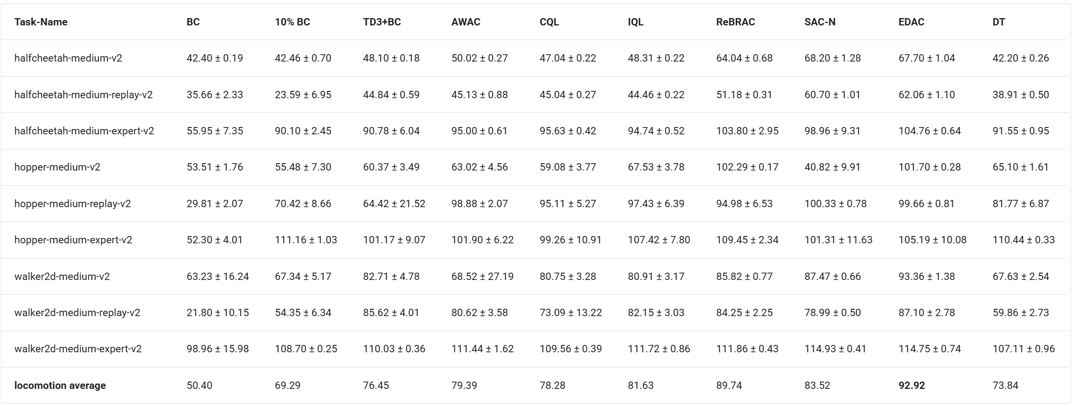
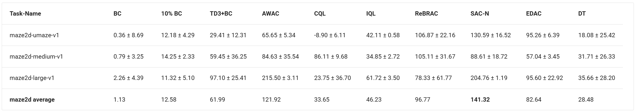
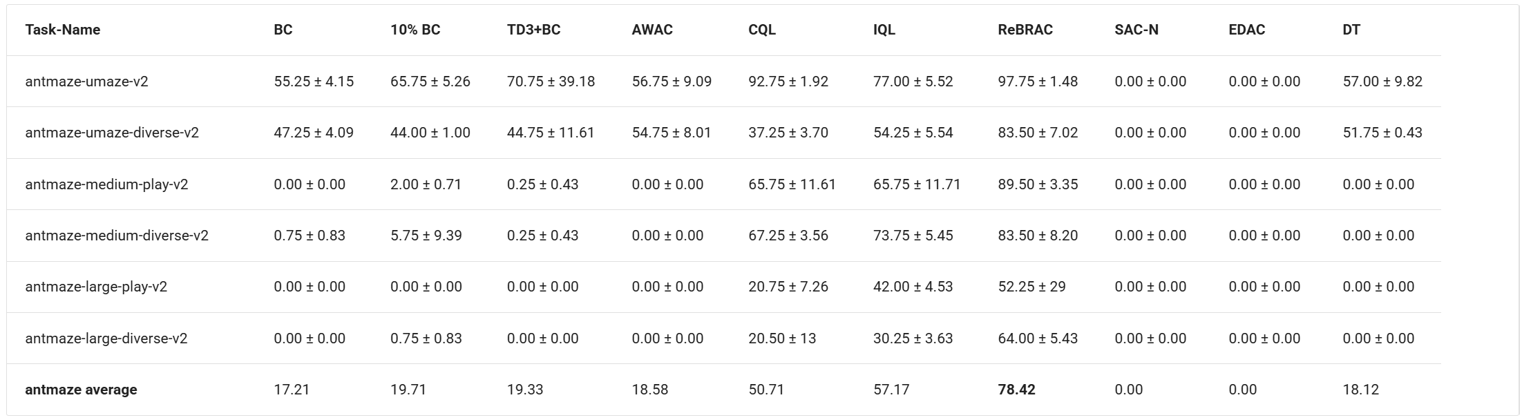
How does Offline RL Perform

Offline RL consistently outperforms BC across standard benchmarks, especially on tasks requiring stitching (like AntMaze). Among the methods discussed, XQL, IQL, and ReBRAC achieve state of the art performance while being computationally faster than CQL.